Introduction

The scientific field of histology is a branch of biology which examines the structure of biological tissues and cells [1]. For this, it is needed to have a visual representation of the tissues and cells. In normal conditions, they have little inherent contrast under a light or an electron microscope. In addition, not all parts of the material is of interest for the study group. Thus, staining techniques are used to enhance contrast and to allow highlighting specific compartments of a sample under a microscope [2].

There is a wide variety of staining techniques and colour configurations [2]. The technique of our interest is indirect immunofluorescence staining. This technique uses the highly specific binding of an antibody to its antigen [3]. Antibodies are Y-shaped proteins which have very specific ends, which are only able to bind with a very specific molecular structure, called its antigen [3]. In indirect immunofluorescence, a primary antibody first binds to the antigen of interest, which is contained in the part of the sample that needs to be highlighted. Then a secondary antibody, which is conjugated to a fluorescent molecule like DAPI, binds to the primary antibody [3]. Thereafter a fluorescent microscope illuminates the sample with light of short wavelength. The light is absorbed by the fluorescent molecule, causing it to re-emit light of longer wavelengths. The re-emitted light is filtered through an emission filter and captured in a detector, which produces an image [5].

We would like to thank our supervisors for proposing this project and helping us develop a solution. The goal of this project is to develop an automated procedure for counting the number of DAPI-stained cell nuclei in an image as well as the number of cell nuclei in tropomyosin-positive myofibers. This ratio is an important parameter in image analysis of in vitro formed myofibres since it is an indicator of how well the cells fused and formed tropomyosin-positive myofibres. The Tissue Engineering Lab is a subunit of the Department of Development and Regeneration of KU Leuven campus Kulak. Their research is focused on skeletal muscle tissue engineering with various applications ranging from the development of cultured meat to regenerative medicine.
We started reading studies about Deep Learning methods, such as pure code methods as DeepCell and U-net [6][7], but also interactive deep learning algorithms such as Ilastik and CellProfiler [6][8]. We took notions of non-machine learning methods, which have special thresholding, edge detection or water shedding implementations [9][10].

Objective

The objective of the project is to develop a consistent process for automated counting of the total number of nuclei and the number of nuclei in tropomyosin-positive fibres in an image in order to calculate the ratio between those two numbers, called the fusion index. The procedure needs to consist of multiple algorithms that detect nuclei and fibres and calculates their positions on the image. The most important goal of the algorithm is not that it is perfect, but that it is consistent and outputs a representative number for the fusion index, since this number is used to compare the fibre formations between different images.

The procedure should be encapsulated in a graphical interface, which needs to have user-friendly features, like processing multiple images, saving workspaces, removing certain colour channels, exporting indicated images and image variables,… The result of the algorithm also needs to be displayed on the interface by showing the image with the counted cells indicated. The user should then have the possibility to manually adjust the indicated nuclei if desired. The whole procedure and interface need to be managed by one executable program written in Python.

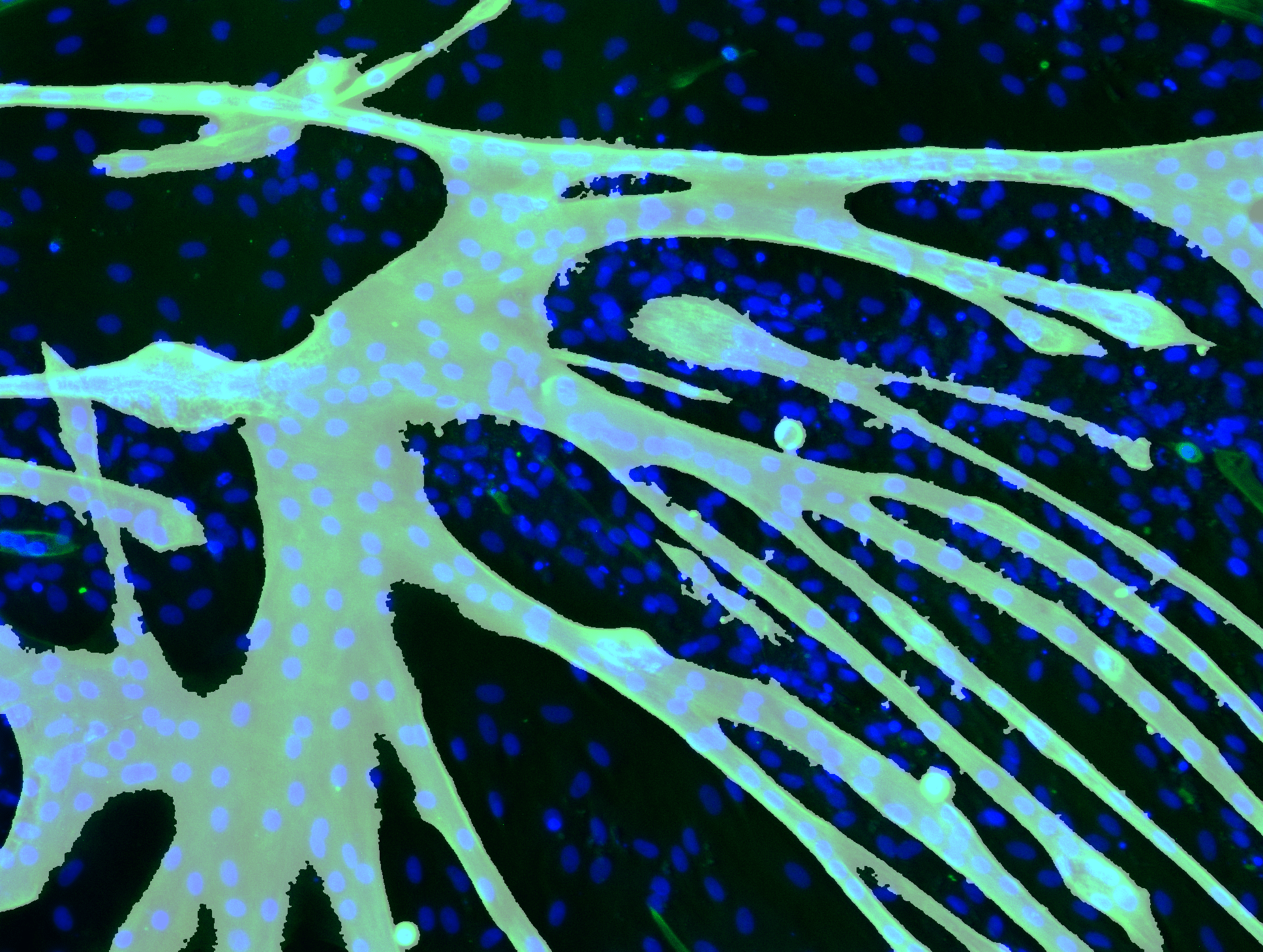
Dataset overview

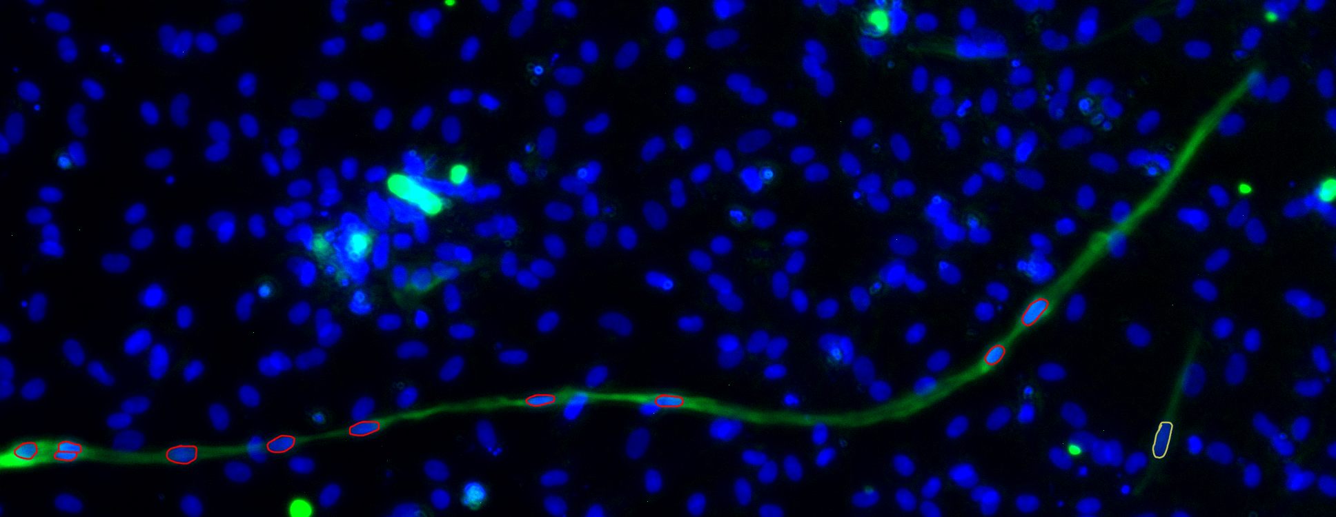
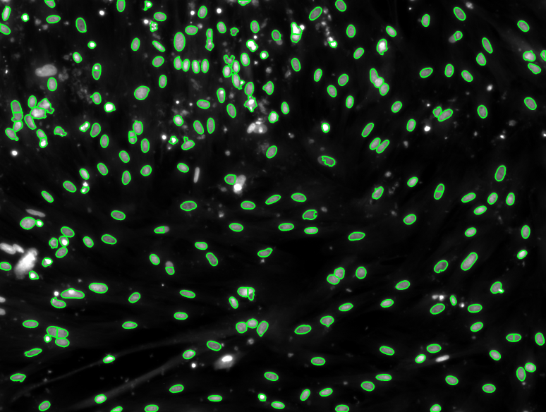
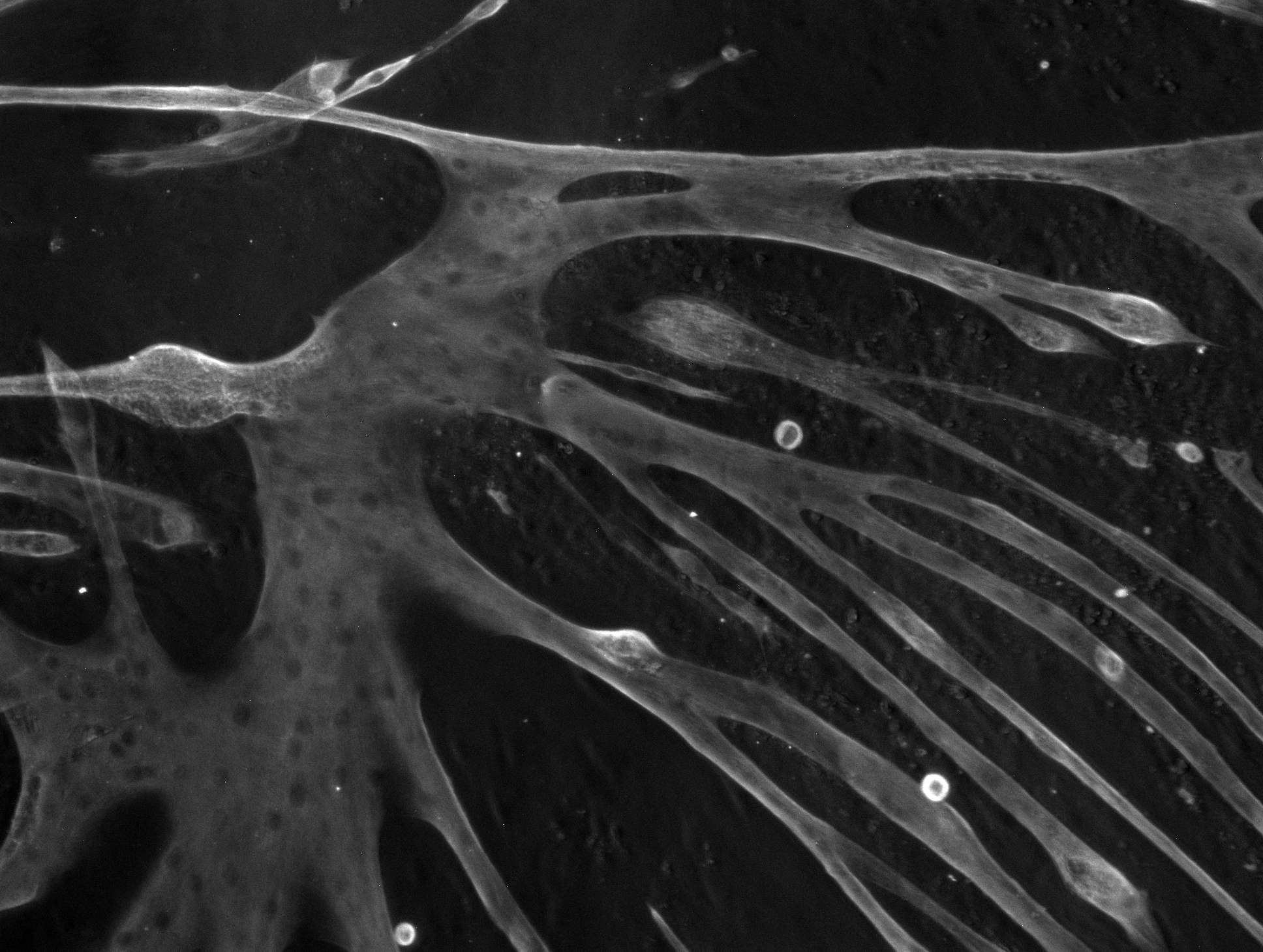
The provided dataset consists of 160 images, where cells and fibres are distinguishable by two different colours, together with semi-automatically counted number of cells. One of the provided images can be seen in Figure 1, together with an extract from the semi-automatically counted data. The nuclei are blue oval shapes, which can be overlapping. Small blue circles should not be counted as nuclei, since these are remains of dead cells. Nuclei that need to be counted as tropomyosin positive, i.e. in tropomyosin fibre, need to be completely inside of the fibre. These nuclei are indicated in red on Figure 1. The nucleus indicated in yellow is not tropomyosin positive, since fibres with less than three nuclei in them are generally not counted as fibre. This last rule can be neglected, since it only has a small impact on the fusion index. Unfortunately, the semi-automatically counted data is not perfectly accurate, which means we should be careful about blindly comparing the outputs of our algorithms to the semi-automatically counted data. An example can be seen in Figure 1. Although the provided data reported 55 tropomyosin positive nuclei, there are in reality only ten. Although this is an extreme case, multiple images can be found with large inaccuracies. In response to this issue our supervisors manually counted and indicated five images exactly. By visually checking how the researchers identify nuclei, we can evaluate our methods.

Name	n	m	r
fKt3-P3-UM-1.2	669	55	8.22%
fKt3-P3-UM-1.3	531	0	0.0%
fKt3-P3-NM-2.3	393	59	15.01%
fKt3-P3-NM-1.2	328	25	7.62%
fKt3-P3-NM-1.1	338	6	1.78%

Evaluation algorithm

An evaluation algorithm will enable comparisons between methods and optimisation of parameters that occur in those methods.

Method evaluation

The evaluation method takes a method and applies it to every image in the provided dataset. Thereafter, it calculates the necessary variables, which include the relative error of the total number of nuclei and the number of tropomyosin positive nuclei, the absolute error of the fusion index and the duration of the algorithm.

Afterwards, the mean and standard deviation of the before mentioned variables are computed and put in a Table 1. The formulas for the relative and absolute error are given in Equation 1, where x the manually counted and targeted number, x̄ the calculated number, \(Δx\) the absolute error and \(δx\) the relative error.

(1) \(\begin{aligned} \Delta x = \bar{x} - x && \delta x = \frac{\bar{x} - x}{x} \end{aligned}\)

Algorithm	\(δn\)	\(δm\)	\(Δr\)	\(t\)
parameter 1	mean% ± sd%	mean% ± sd%	mean% ± sd%	mean  ± sd

n is the total number of nuclei, m the number of nuclei in tropomyosin fibre, r the number of tropomyosin fibres and t the duration of the algorithm.

n is the total number of nuclei, m the number of nuclei in tropomyosin fibre, r the number of tropomyosin fibres and t the duration of the algorithm.

It is preferable to use a relative error for the number of nuclei, since a relative error is normalised. This means every image is represented equally when we take the mean and standard deviation of the relative error. It also enables us to compare errors of different images. It is advisable to use the absolute error on images with less than five tropomyosin positive nuclei because the relative error for smaller numbers of x can become very big, even if the absolute error is small.

Parameter optimisation

When implementing algorithms, we are faced with multiple parameters, such as thresholds or kernel sizes. These parameters influence the way the algorithm separates nuclei and detects fibres. These parameters are mostly chosen arbitrarily, but can be optimised with the evaluation program. The optimisation algorithm is given multiple configurations of parameters and one of the metrics in table 1 to optimise. It then calculates that metric for every configuration and outputs the one where the chosen metric is minimal.

Cell segmentation and image processing methods

Over the course of the project, multiple methods have been researched and tested. In this section we give a small overview of these methods together with their pros and cons. We also motivate our final selection.

Machine Learning methods

Machine learning algorithms can be described as functions with a lot of parameters, those parameters are optimised with respect to a certain goal based on a training procedure. Deep learning is a subfield of machine learning with the special characteristic in how the algorithm is trained. Ordinary machine learning models become better at optimising their functions but they need external feedback to evaluate their output. With deep learning models, the algorithm can use its own neural network to decide whether the prediction is accurate.

Although the performance of nuclei detection by machine learning is overall better, the computation and manual work time is also higher, which is why it is only advised for large datasets which have pinpoint accuracy. In our case, machine learning can only be used if it has been pre-trained by other facilities such as DeepCell, or if the machine learning models have lots of parameters to use like Ilastik or CellProfiler, since we don’t have access to a large dataset of images with indicated nuclei.

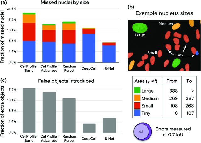
The two algorithms that were found to have the best accuracy are U-Net and DeepCell [6]. Their study is summarised in Figure 2. Unfortunately, U-Net does not have a pre-trained model, it is also slow compared to DeepCell and can use up to ten gigabytes of GPU memory [6]. This is why no tests have been performed using U-Net. In contrast, DeepCell is a better alternative and will be discussed in detail in the next section.

DeepCell

Deepcell is an open source Python library that can be used to train models to predict the location of nuclei. We can call this library directly from Python, in which the graphical interface is implemented. It has user-friendly features to run pre-trained deep learning applications. The DeepCell application of interest is called Mesmer.

Mesmer performs whole-cell segmentation of multiplex tissue data. It needs an image containing both a nuclear marker and a cytoplasm marker. Mesmer is essentially a pre-trained convolutional neural network, but for further details on how Mesmer works, see [11]. Deepcell Applications are models that have been pre-trained for a particular function, meaning that a model has been built using around 25 thousand images [6]. The trained model then becomes a pre-model that can be used for new data. The closer the new data resembles the trained data, the better the predictions are. This is certainly not the best solution as it does not allow for improvements of predictions. The parameters of the model have already been set and cannot be changed. However, DeepCell also contains a post-processing algorithm which is not a machine learning algorithm. This post-processing algorithm further refines the Mesmer prediction using watershed 4.2.3. This watershed algorithm has a dozen adjustable parameters which we can optimise 3.1.

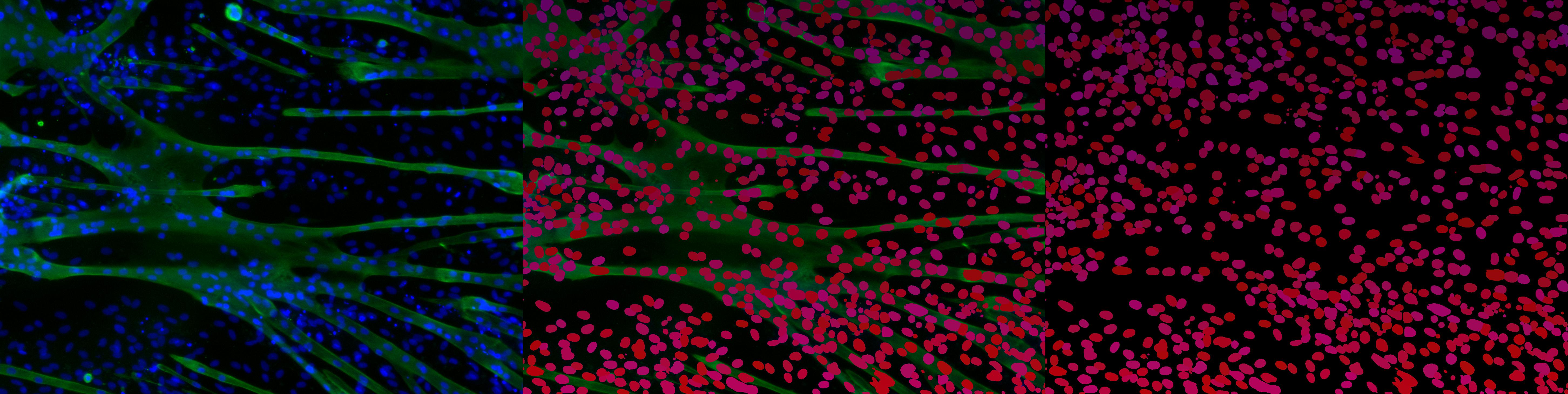
In Figure 3 is an image of the unprocessed, raw prediction made by Mesmer without post-processing. The prediction always finds every oval-like shape in the image, even if they slightly overlap or if parts of the image are darker than others. Problems like missing nuclei in highly overlapping shapes or also falsely indicating dead nuclei, which are a lot smaller, can be partially fixed using the DeepCell post-processing algorithm or even writing an additional post-processing algorithm ourselves.

Overall, We chose deepcell for its ease of use. Deepcell is a library written in python which is also easy to use. The documentation is scarce but still useful and we chose it for the accuracy despite using premodels.

Ilastik and CellProfiler

The second biggest method we tested is Ilastik, an interactive software tool that is easy-to-use for users without much experience but also goes more in depth for people with more knowledge [8]. It has different workflows, which means different sets of algorithms or training modules depending on what sort of machine learning program you need. The two workflows we use for this project are pixel classification and object classification.

Firstly, the pixel classification creates probability maps based on where the cells are in the picture, but it can’t differentiate between different cells that are attached to each other. This is why we need the object classification module that uses a Random Forest algorithm. This works by first smoothing and thresholding the probability maps gained by the pixel classification module. Finally, features are computed based on the users preferences, like intensity statistics or convex-hull-based shapes. The important part is the possibility to implement our own features using a Python template.

The advantages of Ilastik are that it is free to use for experienced users who have implemented their own code and plug-ins, This, coupled with the fact that it can be run from the command line, means that it can be put into a Python script without having to run Ilastik. Ilastik also has a built-in fibre detector. Its disadvantages are mainly the persistence of small errors in the algorithm and the lack of adaptability to different conditions, such as zoomed images.

As another free open-source and well-known cell segmentation program, we shortly researched CellProfiler. It we chose not to use Cellprofiler because there are too many external dependencies that would need to be installed. Furthermore, researchers have not found CellProfiler to be an accurate cell detector [6].

Classic methods

OpenCV is a cross-platform library for developing real-time computer vision applications. It focuses on image processing, video capture and analysis, including features such as face and object recognition. we can combine to count the number of nuclei in an image. The operations that we will use are explained in the following section. Later, we will give the combinations of operations that defines our possible algorithms.

Pixel based ratio method

The most primitive method we developed is one that counts the amount of pixels with blue and green values above a certain number. Each pixel contains three different values between 0 and 255 for the intensity of the blue, green and red colour. Based on experiments, the results were favourable when 4O was the value for both the blue and green intensity. Thus the algorithm counts every pixel with an intensity above 40 for the blue, respectively green colour as a blue, respectively green pixel. If both values are greater than 40, the pixel will be counted as a pixel of a tropomyosin positive cell. Afterwards, the ratio of tropomyosin positive pixels will be checked and compared to the ratio of the given values in the Excel spreadsheet with the evaluation algorithm. Note that the time it takes to compute everything, as looping over an image with dimensions 1936 by 1460 is equally time intensive as looping over 2 286 465 values. The percentage of error for this method was promising (between 3% and 8 %), but it takes about fifteen seconds per picture to compute the ratio, which is too much time when you want to analyse lots of pictures, at least if the error percentage is approximately 5%. As a second attempt at making a simple, but better algorithm, a variant was developed which counts the literal pixel intensities instead of the pixels itself. That means that when a blue pixel for example has an intensity of 189, which is above 40, 189 is added to the total blue intensity instead of 1. The results were not really better than those of the simpler method. It was noticed early on that these both weren’t going to be the final method to count the ratio, because they are fairly primitive methods, but we were interested in how close we could get to good results.

Thresholding

Before we apply a threshold to an image, we need to go through two steps. The first of those is splitting the image into different channels. We basically split the image into three different images tagged b, g and r (for blue, green and red). Then we convert one of those three images to greyscale, dependent of which colour we need (to detect nuclei for example, we would convert the blue image to greyscale). After this step, we can apply a threshold to the image, which now contains only grey pixels with an intensity based on the blue intensity of the pixels in the first image.

There are different thresholding techniques available when using OpenCV. The different options are binary, inverse binary, trunc, tozero, inverse tozero and finally Otsu’s technique [12][13]. The binary technique is the simplest way of thresholding and this is the only thresholding type we use in our final program: it checks the intensity of each pixel and replaces it with zero if the intensity is lower than the threshold value, and 255 if the value is higher. That way the foreground is separated from the background, and we can easily apply different operations on the image. We also tried adaptive thresholding, Otsu’s method and thresholding per 1/16th of the image but found out the binary method is the most trustworthy and consistent method.

Watershed

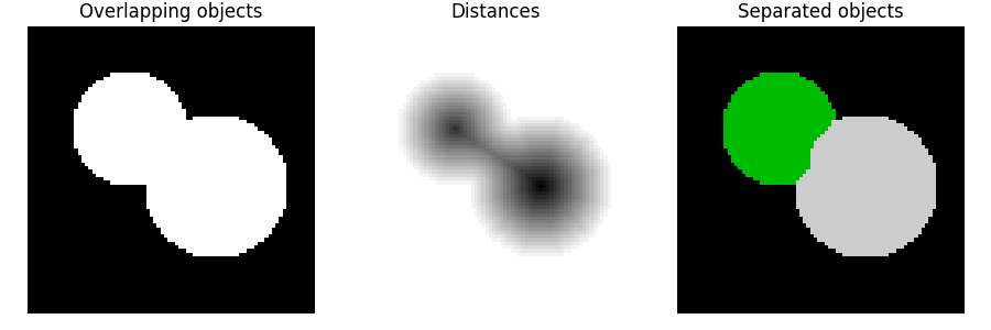
For dividing different cells that are for example touching or overlapping, the watershed method is very useful. It is based on the real life term watershed, which is used to name elevated terrain that divides neighbouring drainage basins. According to [14], there are different ways of applying watershed to an image but the method used in most cases is the ’watershed by topographic distance’ method. It uses a distance map which is an array of the same size as the input image, but instead of the intensity of the pixels it contains the Euclidean distance to the closest background pixel, for each pixel. (The Euclidean distance of a background pixel to the closest background pixel is 0.) Based on that distance map, the algorithm can identify and split different objects, even when they are touching.

Morphological operations

Morphological operations are operations on images that process the image based on shapes. The most basic morphological operations are eroding and dilating. These operations are used to eliminate noise and to isolate or join shapes in an image. The dilate operation convolves a kernel over the image. Each pixel value is replaced with the maximum pixel value of all the pixels surrounding the original pixel. This causes the bright shapes to grow, hence the name dilation. The erode operator does the opposite of the dilate operator. It replaces each pixel value with the minimum pixel value of all the pixels surrounding the original pixel. This causes bright shapes to shrink, hence te name erosion [16].

Combining the erode and dilate operations gives useful results. A dilate operation followed by an erode operation is called closing an image, because this will remove small holes in shapes. After the dilate operation, holes will be filled because the hole pixels are replaced by the bright pixels surrounding the hole. Because of the dilate operation, bright shapes will also grow, which is not always desired. To reset the shapes back to their original sizes, the dilate operation is followed by the erode operation [17]. The opposite operation is opening an image, which is done by first eroding the image, removing small bright ’noise’ from the image, followed by dilating so the big enough objects simply return to their original size.

General selection

As for the second method using OpenCV, that would be a combination of the image processing operations described in the methods section of this paper, we were going to write about which operations we chose to combine and write our final program with. This method was going to be used if OpenCV would be part of the final algorithm, which it probably won’t, so instead we will argument on why the machine learning methods will likely be more efficient. First of all, designing a machine learning program in Python from scratch is not feasible, since we don’t have enough data to our disposal, so the benefits of ’training’ the program are not accessible if OpenCV was chosen as our main method. Another disadvantage would be that a method in OpenCV needs to be written from scratch, and then still have to optimize it, while in an existing program, we can start optimizing the parameters from the beginning. We had some decent results, both analysed visually and using the data available, which can be seen in 4. Most of the cells are correctly highlighted, some cells are ignored and some cells are wrongly split into different cells. As a semi-automatic method this could still be a viable program, but we wanted something working a little better than this.

Graphical User Interface

The implemented algorithms will be encapsulated in a user interface on a desktop application. The use only has to interact with the interface to make use of the automated algorithms. In this section we will only briefly go over the interface abilities, more details can be found in the manual 10.

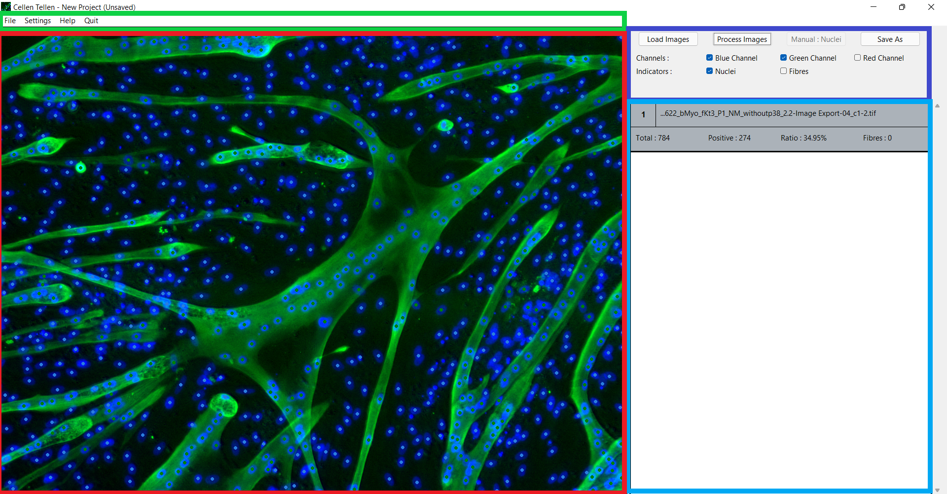
While the program starts up, a splash screen is shown with the credits of all team members and supervisors. The user interface itself consists of four panels, as shown in Figure 5. The green panel shows the menu bar, with capabilities of creating, deleting, saving and loading projects. It also provides some settings for the detection algorithms and contains a Help button which directs the user to the GitHub repository [18].

The dark blue panel is the essential toolbox. There you can load multiple images and process them with the automatic algorithms. It is also possible to select some features of the image displayed in the red panel, such as which colour channels are displayed and whether the automatically or manually indicated nuclei or fibres will be shown.

In the light blue panel there is a table with all the required information about each image. This information consists of the name of the image, the total number of nuclei, the number of tropomyosin positive nuclei, the fusion index and the number of fibres. If you click on the row of a specific image, that image will be displayed in the red panel. The user can zoom and move around in the image with the mouse and keyboard buttons. If needed, the user can manually indicate nuclei or remove indicated nuclei and fibres, which will automatically change the nuclei count and fibre count of that image.

Lastly, it is possible to export the original images with the detected nuclei and fibres indicated on them. The variables of each image can also be exported to an excel sheet.

Implementation

By using a combination of classical methods and Deepcell, It was possible to construct the best suited algorithm for detecting nuclei and deciding if they are tropomyosin positive. An overview of the algorithm is shown in Figure 6. The output of the process is all the positions of the detected nuclei and fibres. Firstly, the DeepCell Mesmer application applies the prediction algorithm and post-process algorithm. Secondly, the fibre detection algorithm produces a mask which we can use to detect whether a nucleus is contained in fibres. Lastly, the algorithm calculates the centre position of every nucleus and decides if it is tropomyosin positive. If desired, the algorithm will also count the number of fibres as well as determine representative points to indicate the fibres in the interface. Every step of the process will now be described in detail with a short note on the time complexity.

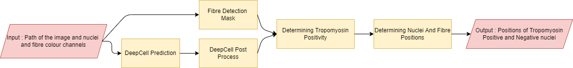
DeepCell Prediction and Post Processing

The DeepCell Mesmer premodel calculates a background, cell interior and cell edge probability for every pixel of the image. The built-in post processing algorithm then collapses this probability map to a segmentation map. This is a two-dimensional matrix with the same shape as the original image. Every position of this segmentation map contains an index, this index refers to the nucleus that the corresponding pixel in the original image is a part of.

The post processing algorithm performs a number of operations which depend on user-given parameters. The most important operation splits up the probability map in separate nuclei based on a watershed algorithm. The distance transform of this watershed algorithm is determined by a neural network [7]. Deciding which maxima become nuclei centres is decided by two parameters. The first parameter decides a threshold value and the second parameter radius of disk used to search for maxima.

After the watershed algorithm, the post processing algorithm removes all detected nuclei smaller than a certain value, which is the third important parameter that we made use of. These parameters were optimised with the evaluation algorithm 3.1 and also by visually checking the output.

The DeepCell prediction and post processing are a lot more time consuming than the next parts of the algorithm, which we have implemented ourselves.

Fibre Detection

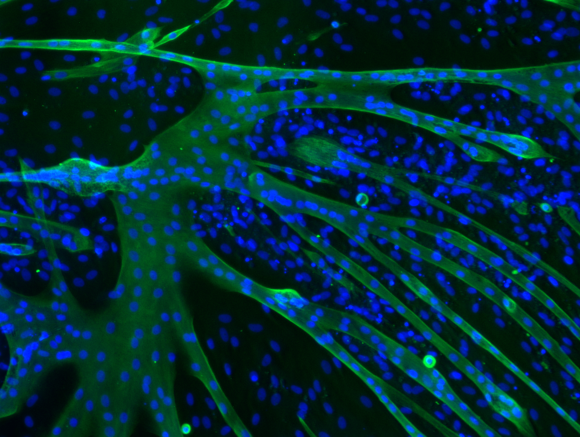
For detecting which cells are tropomyosin positive, we apply the following algorithm. First of all we split the channels of the image and we apply a manual threshold to the channel with the colour of the fibres (green for all images in this project). Then we apply this ’binary mask’ to the green channel. What happens here is that the original pixels are preserved when the corresponding mask value equals 255, and set to 0 if the corresponding pixels in the mask is 0. That way we have a greyscale image with only the green pixels with an intensity above 20 (= the first threshold value). After that first threshold, a few more thresholds are applied, each time being based on the previous one, so that we can start differentiating the foreground from the background. The final threshold is based on the amount of non-zero pixels in the second to last thresholded image, the average intensity of the green channel after the first threshold (with value 20) and the average intensity of the green channel of the original image. That way a kind of adaptive threshold value is calculated based on the original image. To ensure consistent results, a minimum and a maximum value are provided so we dont get unexpected and unuseful output for exceptionally different images. Once we have the thresholded image, we use the opening operation to remove small white noise without changing the size of the fibres themselves. After that, we determine what white objects are fibres and which aren’t. This process uses 3 characteristics of contours of white objects: the perimeter, the area and the radius of the minimal enclosing circle. The area and the perimeter are used to determine if a white object is big enough to be seen as a full fibre, the radius of the enclosing circle will be bigger for longer objects with a rather small area than for circular blobs with a big area (which usually aren’t fibres). Once the white objects that are no fibres are removed, the image gets closed to fill in little holes in the fibres. To fill in bigger holes in the fibres, which are present to a large extent, the image is converted and a similar technique is used to the one used to remove small noise: if a hole (now white, thus foreground) is small enough, it gets filled in, or, as you could say, simply removed from the image. By afterwards inverting the image again, we get the fibres without the holes, which can be seen as black noise.

Determining Nuclei Positions

It is necessary to determine the centre positions of the nuclei to indicate them in the interface. Furthermore, if we know all the pixels that contribute to a nucleus, we can, in combination with the fibre detection mask, decide whether a nucleus is tropomyosin positive.

Firstly, it is necessary to find all the pixels that contribute to a nucleus. Since the output of the DeepCell post processing is a segmentation map, we are forced to utilise a NumPy function which finds all pixel coordinates of a certain value.

Secondly, from these coordinates we calculate the mean x− and y−value and use this mean point as the centre of our nucleus. Since the nuclei are concave, this mean point will always be inside of the nucleus.

Lastly, if the portion of the area that overlaps with fibre reaches a certain threshold, we count the nucleus as tropomyosin positive. Theoretically, a nucleus needs to be fully inside of the fibre to count as tropomyosin positive 2, so the threshold value should be one. Practically, the fibre and nuclei detection will never be perfect, due to distortions and noise in the original image on the pixel level. Therefore a threshold of a little less than one is used.
Although there are certainly algorithms with the same functionality which perform less operations than the explained one, they might not be faster. Our algorithm makes use of NumPy operations as much as possible, which are very fast.

There are some additional details that speed up the algorithm. For example, the DeepCell post processing will number the detected nuclei from top to bottom in the segmentation map. This means we can be very certain that two nuclei with succeeding indices will be very close in vertical position, since there are always a lot of nuclei spread around the image. Therefore, we only have to scan a small band above and below the previous nucleus to find all pixels contributing to the next one. This speeded up the algorithm about seven times.
All sorts of these small or big improvements make the duration of this part of the process negligible compared to the DeepCell prediction and post process.

Determining Fibre Positions

The program also encapsulates a mechanism to count and indicated fully disconnected fibres if desired. This algorithm also makes use of the fibre detection mask.

Splitting the mask up in disconnected parts is straight-forward, since the mask is binary we can apply the OpenCV operation findContours which gives a list with all contours in the image.

Finding visually logical representative points to indicate the fibres is less straight forward. The problem is that just taking the geometrical centre point of the fibre will most likely not be located inside of that fibre, since fibres are rarely concave. The goal is to find a point which clearly indicates what fibre it represents. The first of our conditions for these points is that they should be located deep inside of the fibre, i.e. far away from the edge. Secondly, we want it to be close to the geometrical centre of the fibre and thirdly, the point should not be too close to the edge of the image.

To find the point that optimally meets our conditions, we have established a utility function in Equation [eq:utility]. Firstly, we apply a distance transform which gives the smallest distance to the background for every fibre pixel. We then eliminate all pixels that are less than the 80th percentile away from the edge. From the 20 percent furthest pixels we find the point where the utility function in Equation [eq:utility] is minimal. In this equation, d_c is the distance to the geometrical centre of the fibre and d_b is de distance to the closest background pixel. Because of the d_c² term, the selected pixel will be close to the geometrical centre.

Notice that, even though we have already eliminated pixels close to the edge of the fibre, we still have a term d_b³ in the utility function, this is because

Note that d_c is raised to the second power in the utility function, since receiving the value of d_c required taking the square root of d_c², which is very time consuming. Since squaring is a monotone operation on the positive domain, this will not affect the position of the minimum value. d_b is raised to the third power. Firstly, this makes sure that both terms are of magnitude. Secondly,some images have a type of hub where a lot of fibres are connected to, like in the example image of the fibre detection algorithm 16. The geometrical centre of these hubs if often not a representative point of the fibre. A more representative point is the centre of this hub, which is often very far from the edge. In these cases, the  − d_b³ term will take the upper hand and thus the centre of these hubs are taken as the representative point.

\[\begin{aligned} f\left(x, y\right) = d_c^2 - d_b^3 \label{eq:utility} \end{aligned}\]

To impose the third condition, i.e. the representative point must not be too close to the border of the image. We just add a black line at each border of the image. These black lines will be taken into account as background in the distance transform. Since we eliminate points that are too close to the background, points that are too close to the border will now also be eliminated.

Since representative points don’t not need to be very accurate, we can scale the dimension down by two, which will speed up the algorithm four times.

These representative fibre points together with the nuclei positions are then sent back to the user interface.

Performance boost

An important issue in creating an accurate algorithm is the time complexity and duration. We were able to optimise the self-implemented algorithms by narrowing the number of calculations or using very fast libraries such as NumPy. The time complexity of these algorithm is now negligible to the time complexity of the DeepCell prediction and post processing. Since we are not able to adapt the DeepCell code, we attempted to make more optimal use of the computation power of our computers.

A possibility to improve performance is to make use of multithreading, where multiple independent pieces of code can run in parallel. The central processing unit (CPU) quickly switches between different pieces of code and executes them. Because this is done so quickly, it creates the illusion of the pieces of code being run in parallel [19]. The important part of multithreading is to make sure the user interface is still interactive when the images are being processed. This is because the user interface is run in parallel with the processing of the images. The second benefit of multithreading is that it gives a performance improvement, reducing the execution time off the full process for one image from 20 seconds to 16 seconds.[1]

A different way of making efficient use of computation power is to let processes run on the graphics processing unit (GPU). DeepCell uses TensorFlow, and TensorFlow supports running processes on a nvidia graphics card by using CUDA, a driver created by nvidia to let processes run on a modern nvidia graphics card [20][21]. Since processes are then running on the GPU, it is not possible to continue using multithreading, since this can only be used in combination with the CPU. Using the GPU will greatly reduce execution time of the full process from 20 seconds to 6 seconds.[2] However, it is required to posses a nvidia graphics card and have CUDA installed. The program is fully prepared for GPU optimisation, once CUDA is installed, the program will automatically start using the GPU. The installation manual of CUDA can be found on the GitHub repository [18].

Results

As a recap, our objective was to separate nuclei, count them and indicate them accordingly. In this section, It will be shown how the final configuration faired against 25 images. The amount of images were arbitrarily chosen as what normal operation would look like. Ideally, the time taken per image should be more or less the same. Secondly, it will also be shown how accurate the final configuration is against our pre-determined numbers of nuclei. Ultimately, The result shouldn’t deviate more than two percent.

Name	time(sec)	timeperimage(sec)	accuracy(%)
First test	669	55	8.22
Second test	669	55	8.22

In this table, it is clear as day that, the time …. the accuracy …..

As you can see there is a clear difference between running the program with CPU and GPU. The time needed to process one image is ..

These are our results compared to the medical group with a standard deviation of only three people. We took five photos that are very different in photo quality and nuclei distribution so we have our edge case results plus an average photo. We of course tested this on way more photos and visually come to the conclusion it indeed worked on all of them. It is clear that our goal of 2 percent within the green nuclei percentage has been reached. Together with the fact that we brought our time complexity of our program down to … seconds on a slow computer. As such, we are very happy with our results.

Name	(Percentage green nuclei by the medical group (±sd) in %	Our results in %	Total cells
First photo	36, 34 ± 1, 82	35, 96	805
Second photo	55, 82 ± 1, 42	55, 95	422
Third photo	81, 98 ± 1, 11	80, 43	390
Fourth photo	53, 94 ± 0, 62	53, 85	330
Fifth photo	35, 31 ± 1, 01	33, 40	196

Conclusion

Reflection and improvements

In this last section we will go over some of our reflections over the course of the semester as well as some possible improvements of the nuclei detection.

There could have been improvements in the communication with our supervisors. For example, we have create a performance boost by using a nvidia graphics card, which most of our supervisors don’t have. It would be far more beneficial to optimize our program to be able to run on all possible graphics cards. The time spent on researching for a faster solution using nvidia, could be well spent otherwise.

Because of our concerns around the dataset, we had a hard time testing our algorithms in the beginning of the semester. We later asked for five images, where the counted nuclei were indicated. This gave us a way to visually verify the correctness of the algorithms. We thank our supervisors for this, although we should have asked these images sooner in the semester. It would’ve also been helpful to have more exactly counted images so that we could also compare our algorithms numerically to a big batch of images.

We spent the first half of the semester researching and testing detection methods, before making the selection to use DeepCell, partially because of our setbacks concerning the given dataset. This means that we believe using DeepCell was the correct selection. But a consequence is that there are certainly more post processing improvements that we could have implemented given enough time.

Some of these post-processing improvements could be :

• Implementing the rule where fibres with less than three nuclei can be eliminated. However, this rule is not always followed by the researchers and would not have a big impact on the final output of the algorithm, since we are talking about a handful of nuclei per image.

• In some images, there is a blue shine around the fibres. This is only visible if the green channel is switched off. The DeepCell algorithm will sometimes detect these shines as nuclei. A possible improvement would be to detect and remove these wrongly identified nuclei. This will also have only a small impact on the macroscopic output of the process. The shine is also hard to detect, since the shape and intensity is different from image to image.

• The DeepCell prediction works well for segmenting clumps of a handful of nuclei, but clumps with more than a handful, it will not correctly identify all nuclei. We could improve this by applying a type of convexity-detection algorithm, which will identify convexity defects. These convexity defects have a strong relation to the number of nuclei in the clump, since a single nucleus is mostly concave. Implementing this method was complex and would also wrongly identify multiple nuclei in shapes that only consisted of one nucleus, since nuclei are not always fully concave. The number of clumps with more than a handful of nuclei is also very small.

These improvements will not have a big effect on the macroscopic output of the algorithm. Furthermore, it is also not needed to have an algorithm that counts the nuclei exactly. Firstly, the most important output is the fusion index. This ratio is only slightly dependent from these improvements. We can verify this by remembering the pixel ratio method 4.2.1, which already gave us a decent approximation of the fusion index. Secondly, like explained earlier, the goal of the project was to have a detection algorithm that outputs a representative and consistent ratio, which is not necessarily one that is exact.

authors: Quentin De Rore, Ibrahim El Kaddouri, Emiel Vanspranghels, Henri Vermeersch
Supervisors: Desmond Kabus, Maria Olenic, Rebecca Wüst

References

1. Histology. Wikipedia. Accessed on 23-10-2021.
2. Staining. Wikipedia. Accessed on 23-10-2021.
3. Immunofluorescence. Wikipedia. Accessed on 23-10-2021.
4. Antibody. Wikipedia. Accessed on 23-10-2021.
5. Fluorescence microscope. Wikipedia. Accessed on 23-10-2021.
6. Juan C. Caicedo, Jonathan Roth, Allen Goodman, Tim Becker, Kyle W. Karhohs, Matthieu Broisin, Csaba Molnar, Claire McQuin, Shantanu Singh, Fabian J. Theis, and Anne E. Carpenter. “Evaluation of deep learning strategies for nucleus segmentation in fluorescence images.” Cytometry Part A, 95(9):952–965.
7. Kudo Graf Covert Van Valen Moen, Bannon. “Deep learning for cellular image analysis.” Nature Methods, 16(12):1233–1246.
8. Stuart Berg, Dominik Kutra, Thorben Kroeger, Christoph N Straehle, Bernhard X Kausler, Carsten Haubold, Martin Schiegg, Janez Ales, Thorsten Beier, Markus Rudy, Kemal Eren, Jaime I Cervantes, Buote Xu, Fynn Beuttenmueller, Adrian Wolny, Chong Zhang, Ullrich Koethe, Fred A Hamprecht, and Anna Kreshuk. “ilastik: interactive machine learning for (bio)image analysis.” Nature methods, 16(12):1226–1232, 2019.
9. Amin Gharipour and Alan Wee-Chung Liew. “Segmentation of cell nuclei in fluorescence microscopy images: An integrated framework using level set segmentation and touching-cell splitting.” Pattern Recognition, 58:1–11, 2016.
10. Walker Johnson Abdolhoseini, Kluge. “Segmentation of heavily clustered nuclei from histopathological images.” Scientific Reports, 9(1).
11. Noah Greenwald, Geneva Miller, Erick Moen, Alex Kong, Adam Kagel, Christine Fullaway, Brianna McIntosh, Ke Leow, Morgan Schwartz, Thomas Dougherty, Cole Pavelchek, Sunny Cui, Isabella Camplisson, Omer Bar-Tal, Jaiveer Singh, Mara Fong, Gautam Chaudhry, Zion Abraham, Jackson Moseley, and David Valen. “Whole-cell segmentation of tissue images with human-level performance using large-scale data annotation and deep learning.” 03 2021.
12. Basic Thresholding Operations. Accessed: 2021-11-02.
13. Thresholding (Image Processing). Accessed: 2021-11-02.
14. Watershed (Image Processing). Accessed: 2021-11-02.
15. Watershed Segmentation. Accessed: 2021-11-02.
16. OpenCV: Erosion and Dilation. OpenCV Docs. Accessed on 29-10-2021.
17. OpenCV: Morphological Operations. OpenCV-Python. Accessed on 29-10-2021.
18. GitHub: Cellen tellen. Accessed: 2021-12-16.
19. Computer Architecture: Multithreading. Accessed: 2021-12-16.
20. Compute Unified Device Architecture. Accessed: 2021-12-16.
21. Tensorflow: GPU Support. Accessed: 2021-12-16.

Appendices

In the appendices we have included the interface manual, the subject integration, the responsibilities of each team member, the task structure and the ganttchart.

Cellen Tellen interface manual

This section contains an explanation of the features implemented in the user interface. It can also be found on the GitHub repository together with the python scripts and installation manual .
The user can load (additional) images with the Load Images button. These images can be imported from anywhere on the computer. The names of the images will be shown in a table together with the number of indicated nuclei, the number of indicated tropomyosin positive nuclei, the fusion index and the number of indicated fibres. All these numbers will be set at zero after loading the images. The user can click on an entry of the table to display that image in the imagewindow. Under the buttons at the top of the screen, it is possible to select which colour channels of the picture are displayed (Channels), as well as select whether the currently indicated nuclei or fibres will be shown (Indicators). If at least one image is loaded, the Process Images button will appear. This button runs the nuclei detection and, if desired, the fibre detection algorithm and starts overwriting all currently indicated nuclei (and fibres, if desired) of all the images in the table.

To interact with the displayed image, the user can use the mouse buttons or keyboard buttons. If the user wants to zoom in on the picture, they need to use the mouse wheel or the + and - buttons. To move the image around, the user can hold down the middle mouse button or use the arrow keys on the keyboard. Indicating a new nucleus or fibre happens with the left mouse button. Left-clicking an existing nucleus will transfer it from a tropomyosin positive nucleus to a negative one or vice versa. Right-clicking an existing nucleus or fibre will remove it. While performing these actions, the variables in the table will change for that image. Switching between interacting with the nuclei or the fibres can be done with the third button at the top of the screen (Manual : …). It is only possible to select to interact with the nuclei if the indicated nuclei are also being shown, which can be selected below the buttons (at Indicators). Likewise, it is not possible to interact with the fibres if the indicated fibres are not being shown.
The user can save working spaces in projects. Initially, after starting the program, a new empty and unsaved work space is created in which the user can start loading images. Creating a new project folder and saving the current space in that folder is done by choosing Save Project As in the File menu. After providing a name for the project, the current working space will be saved in that folder.

Loading a project folder can be done directly from the Recent Projects option in the menu as well as from the Load From Explorer option in the menu. This option will guide the user to the folder where all the saved projects are located. Choosing one of the project folders will load that project. In the File menu, it is also possible to delete the current project or start a new empty project (make sure to save the current working space or project before doing this). Finally, the option Load Automatic Save in the File menu will load the latest automatic save.

After loading a project folder or saving the current working space to a project folder, the user will now be working inside of that project. The name of the current project is contained in the title of the window. This title also indicates whether the current working space or project is unsaved. If the user is working inside of a project, it is possible to save the current working space immediately to that project by clicking the Save button at the top right of the window.

All projects are saved in one folder which is automatically created by the program, the user is expected to only alter these projects folders through the interface. When saving a project, an excel sheet will also be created, which contains the relevant variables for each image like the total number of nuclei, the number of tropomyosin positive nuclei, the fusion index and the number of disconnected fibres. It is possible to also save altered images, these are the original images with the detected nuclei and fibres indicated. Both the excel sheet and altered images can be found in the projects folder after saving the project.
In the Settings menu, available in the menu bar, there are a number of options.

• It is possible to indicate which channels are occupied by the nuclei and the fibres. The automatic nuclei and fibre detection is based on these selections.

• The user can indicate how long the autosave interval is, this is the interval between automatically saving the current project to the automatic save folder.

• It is possible to enable saving altered images when saving projects. These altered images are the original images with the detected nuclei and fibres indicated on them.

• One of the performance boosting functions of the program is multithreading. The number of threads can be chosen from 5 to zero (zero means no multithreading, this will temporarily block the program when running the process). It is advised to set the number of threads to one when using GPU optimisation.

• Since it is not always desired to count and indicate the fibres, this functionality can be switched off.

• If desired, the user can adjust the Small objects threshold which is used to remove dead cells by eliminating nuclei smaller than this threshold.

Subject integration

Our project involves some knowledge beforehand that we learned throughout our study at Kulak. First we have the subjects that are essential, these are the ones that are required to complete the project and make a decent scientific paper:

• The first subject is ’Beginnings of programming in Python’. We need the basics of programming before we can make a application or an interface that satisfies the customer. Together with the overall better understanding of main concepts, for example object oriented programming or using different libraries depending on each situation, the subject also explained time complexity and memory usage for programs and algorithms, which are huge factors in our end result because this will mainly influence how the customers grade our program.

• The next course is statistics, it is obligatory for researching data and summarizing our results in tables. See Table 1 for an example on how we use statistics to research which algorithm is the most efficient. We also use it as a key factor to compare our data to the semi-automatically counted data, using factors like mean and standard deviation. A lot of algorithms also use statistical analysis. Otsu’s thresholding method, for example, chooses a threshold value by maximizing the variance between background and foreground.

• In the subject of numerical mathematics, we talked in depth about absolute and relative error. We also discussed the problems with these errors, like bad behaviour for low values of x in a relative error.

• The last three courses that are necessary for the project are ’Problem solving and developing’ one, two and three. These courses are fundamental to engineering and have learned us how to write papers, practically search for solutions and work in teams. These courses are used for everything throughout the project from infrastructure to layout.

• Most OpenCV operations apply specific kernels to an image. These kernels are two-dimensional matrices that update a pixel value by combining the surrounding pixel values based on the values in the kernel. A notion of linear algebra will be enough to understand how these operations are performed and how they combine.

The following courses are not needed but do help a lot with different uses. All maths related subjects are used to learn about these different algorithms and OpenCV operations and how to use them. These subjects also teach logical reasoning, which is essential to problem solving. We’re not going to discuss each subject in depth because our project doesn’t particularly focus on the maths side, but more on the implementation of these algorithms.

[1] All timings are done with an Intel Core i7 CPU and an Nvidia GeForce 1650 Ti GPU

[2] All timings are done with an Intel Core i7 CPU and an Nvidia GeForce 1650 Ti GPU