Introduction

In the pursuit of approximating vibrations, the Fourier transform serves as a vital tool. These oscillations can also be expressed as combinations of trigonometric functions. By utilizing a limited number of amplitude measurements, we can construct an approximation of the vibration. However, the accuracy of this approximation improves with an increased number of measurement points. Our exploration begins with an extensive elucidation of Fourier analysis, encompassing the Fourier series and its application in function approximation. Subsequently, we delve into the Fourier transform, accompanied by a concise method for its execution. Following this, we expound on our program’s implementation, underpinned by theoretical insights, leading to the findings presented in this article.

Fourier Analysis

The core concept behind Fourier analysis revolves around expressing real-variable functions as linear combinations of functions derived from a set of standard functions. The Fourier series is employed to approximate periodic functions by means of a summation of sinusoidal components. Conversely, the Fourier transform is employed for approximating general non-periodic functions. Our emphasis primarily lies in the application of the Fourier series, and thus, the accuracy of our approximations may be limited when dealing with non-periodic functions.

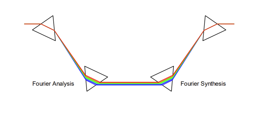
To illustrate this concept more vividly, consider the analogy of two prisms. The first pair of prisms has the ability to disassemble light into its constituent frequencies (colors), a process analogous to Fourier analysis. Subsequently, a second pair of prisms can recombine these frequencies, demonstrating This is called Fourier Synthesis.

Linear combinations and orthogonality of functions

In order to approximate a continuous function effectively, it is imperative to possess a comprehensive set of standard functions. Among these standard functions, one that finds consistent utility in applications involving Fourier transform or Fourier series is the weight function denoted as \(\omega\). For the sake of simplicity, we will assume that this weight function is uniformly equal to \(1\). Furthermore, in our computational framework, we frequently employ the fundamental concepts of orthogonality and norm, which will be elaborated upon in subsequent sections.

However, the significance of orthogonal functions should not be underestimated. When a basis function, drawn from the ensemble of standard functions, exhibits orthogonality, it offers a compact and distinct representation.

Suppose you have a function \(f(x)\) and you want to approximate it using 3 basis functions \(g_1(x), g_2(x), g_3(x)\). then:

As you can observe, there are numerous coefficients, which grow exponentially as the number of functions increases, and they are also non-unique. If the functions were orthogonal, all composite functions would be zero. The set of coefficients would also be unique for each function, leading to the following relationship:

Why would they be zero? We select the basis functions in such a way that their multiplication results in zero. However, this must hold true for all values and all basis functions, hence the need for integration.

• Two functions, \(f\) and \(g\), are orthogonal if and only if

  \[<g,f>=\int_a^b f(x) g(x) \omega(x) dx=0\]

• The norm of a function \(f\) is defined as

  \[||f|| = \sqrt{<f,f>} = \sqrt{\int_a^b f(x)^2 \omega(x) dx}\]

• A function can be expressed as a linear combination of orthonormal functions.

  \[f=a_1 f_1+a_2 f_2+\ldots + a_k f_k\]

  This is the set of orthonormal functions on an interval \([a,b]\).

• We refer to this set of functions as orthonormal if for all i and j, it holds that:

  \[<f_i,f_j> = \left\{ \begin{array}{r@{\text{ als }}l} 0 & i\neq j\\ 1 & i=j\ \end{array}\right.\]

• The coefficients of these linear combinations for \(i \in \{1, \ldots, k\}\) can be expressed as:

  \[\label{eq:orthonormaal} {a_i=\int_a^b f(x) f_i(x) \omega(x) dx = <f,f_i>}\]

Function Distance

Once we have both the approximated function and the original function, we can evaluate the quality of the approximation by assessing the proximity or distance between the approximated and original functions.

This condition should not hold for just one specific value of the two functions but for all values across the functions. Ultimately, we can conclude that the smaller the (quadratic) area between the two functions \(f\) and \(g\), the smaller the margin of error between these two functions. If we now incorporate all of this into the Euclidean distance function, we obtain the following:

We already know that we can express a certain function \(f(x)\) as a linear combination of other functions:

Let’s denote the function we want to approximate as \(g(x)\). Then, it follows that:

So, the better the approximation, the smaller the margin of error, and consequently, the smaller the distance between the two functions.

Approximating a Set of Data Points

We can also approximate functions based on a set of (function) values. Let’s assume that these function values are evenly spaced within an interval \([a, b]\). This interval is divided into \(n\) equal subintervals. In doing so, we obtain equidistant points (points that are evenly spaced from each other):

This allows us to approximate the function \(f\) at the measurement points \(f(x_i)=y_i\). Consequently, the number of measurements is directly proportional to the accuracy of function \(f\) and, by extension, the accuracy of the coefficients \(a_j\).

Fourier Transformation and Information Compression

Compression

Assuming we need to store a list of numbers \(y_0, y_1, \ldots, y_n\), we aim to compress this function. To illustrate how it works, let’s consider a ‘simple’ example. We take the function

with \(\omega = 6 \cdot 2\pi\) rad \(s^{-1}\). Applying the sinusoidal Fourier series formula,

we find that \(a_k = b_k = 0\) except for \(b_6\), which is \(3\) in this case. We can express this function in the amplitude-phase as,

with \(\omega = 6 \cdot 2\pi\) rad \(s^{-1}\). The Fourier-transformed function \(G_1\) can be represented as pairs of \(c_k\) values and \(\phi\) values (phase).

Normally, the time signal \(g_1\) contains infinitely many points (pairs of time and amplitude). With the Fourier transformation, we compress this information into the function \(G_1\), which must contain the following information: frequency along with its associated amplitude and phase shift.

Hence, by utilizing Fourier transformation, we can represent a composite function in an alternative manner, resulting in significant computational savings. Conversely, we can also perform the reverse process, transforming a Fourier-transformed function back into a regular function. For more intricate functions, we can introduce minor adjustments or modifications within the Fourier-transformed function and subsequently revert it to its original form.

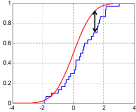
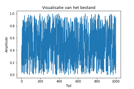
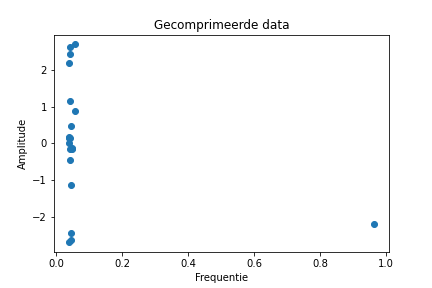
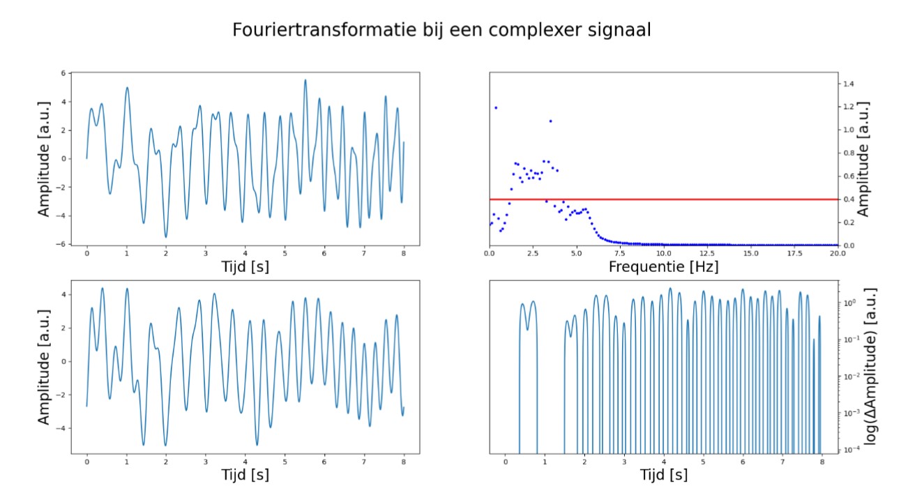
Figure 1 here below displays an arbitrary function, while Figure 2 presents its corresponding Fourier-transformed function. By manipulating this function, for instance, by selecting amplitudes exceeding 0.4, and reconverting it into the original function, we obtain Figure 3. The last Figure serves to visually illustrate the disparity in amplitudes between the original function and the modified version.

Fourier Series

A randomly periodic function can be expressed as a linear combination of basis functions. In this chapter, we will use the sine and cosine functions as our basis functions.

Several conditions for this concept are: [@Drichlet]

• The function \(f\) must be bounded within a specific interval.
• The function \(f\) may have a finite number of discontinuities within a bounded interval.

Fourier Series - Sine-Cosine Formula

First, let’s enumerate the set \(A\) of basis functions, along with our weighting function:

We expand the set \(A\), causing it to become infinitely large:

Now, we can approximate a specific function \(f(x)\) by creating a linear combination of these basis functions. Consider the following formula within the interval \([-\pi, \pi]\), for all \(k \in \mathbb{N}_0\):

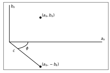
Fourier Series, Amplitude-Phase Formula

We can transform the sine-cosine formula into an amplitude-phase formula. Let’s start with the amplitude-phase formula, from which we will derive the sine-cosine formula:

We can visualize this transformation by representing the \(a_k\) values on the x-axis and the \(b_k\) values on the y-axis. Then, \(c_k\) will be the length of the line from the origin to the point \((a_k, b_k)\). The phase \(\phi_k\) can be considered as the angle between the x-axis and the line \(c_k\) .

To begin the transformation from cosine to the amplitude-phase formula, we can utilize the sum and difference angle identities for trigonometric functions:

Additionally, it’s important to note that the cosine function is an even function, while the sine function is an odd function, which means \(\sin(-\theta) = -\sin(\theta)\) and \(\cos(-\theta) = \cos(\theta)\). Applying these identities and rewriting, we obtain:

where \(a_k = c_k \cos(\phi_k)\) and \(b_k = -c_k \sin(\phi_k)\)

If we calculate \(a_k^2 + b_k^2\), we have:

And for the ratio \(\frac{b_k}{a_k}\), we get:

This formula is more convenient to work with since it involves one less term than the previous formula. The pairs of sine and cosine can be expressed as a single sinusoid with a phase shift, analogous to the conversion between orthogonal (Cartesian) and polar coordinates.

Here, \(c_k = \sqrt{a_k^2 + b_k^2}\) and \(\phi_k = \arctan\left(\frac{b_k}{a_k}\right)\), with \(c_k\) and \(\phi_k\) as polar coordinates.

Implementation

Introduction

In this chapter, we will translate the theory we have discussed into reality. Fourier analysis is not straightforward to perform manually. Therefore, we can enlist the help of computers to carry out these operations. Speed is crucial to efficiently apply the analysis in various applications. In this chapter, we will explain how our team attempted to convert pen-and-paper calculations into Python code.

Calculate Values

The function calculate_Values in our program is the simplest function we use. You need to provide three numbers as input: \(a\), \(b\), and \(n\). These numbers represent the starting value, the ending value, and the number of values you want in the interval, respectively. You will receive a list with n+1 equidistant points between \(a\) and \(b\) as output. For example, if you input \(a=5\), \(b=10\), and \(n=5\), the output will be: \(5,6,7,8,9,10\).

def calculate_Values(a, b, n):
    valueList = []
    for k in range(n + 1):
        x = a + k * ((b - a) / n)
        valueList.append(x)
    return valueList

This function essentially divides the interval \([a, b]\) into \(n+1\) equally spaced points and returns them as a list.

Fourier Series

The function fourierSeries calculates the \(a_k\) and \(b_k\) values that will be important in other functions. The calculation of the \(a_k\) and \(b_k\) values is done here using the summation given in previous sections.

def fourierSeries(y, n):
    ak_coefficients = []
    bk_coefficients = []

    x = sp.symbols('x', real=True)
    valueList = calculate_Values(-float(np.pi), float(np.pi), len(y))

    for k in range(n):
        ak = 0
        bk = 0
        for l in range(len(y)):
            ak += y[l] * np.cos((k + 1) * valueList[l]) * 2 / len(y)
            bk += y[l] * np.sin((k + 1) * valueList[l]) * 2 / len(y)

        ak_coefficients.append(ak)
        bk_coefficients.append(bk)

    return ak_coefficients, bk_coefficients

You need to provide a list of amplitude values (\(y\)) and the desired number of index values (\(n\)) as input. The output is a nested list containing both \(a_k\) and \(b_k\) values, making them accessible and distinguishable for use in other functions.

Read WAV

The readWAV function allows for the reading and conversion of .wav files into usable data. The only parameter here is the path of the .wav file, and the output is also a nested list, containing a list of time values and a list of amplitude values.

Complex Fourier

The complexFourier function works similarly to the FourierSeries function but does not return a list of \(a_k\) and \(b_k\) values. Instead, it returns a list of amplitudes \(c_k\) and a list of phase shifts \(\phi_k\).

\(c_{k}\) Values and Phase Shift

We have computed the \(c_k\) values based on the \(a_k\) and \(b_k\) values. With these values, we can reconstruct the amplitude using the following formula:

We initiated this process by using the code we had developed for fourierSeries. Consequently, we obtained our \(a_{k}\) and \(b_{k}\) values. Subsequently, we substituted these values into the equations for \(c_{k}\) and \(\phi_{k}\), which we then placed into a list for retrieval and used them to reconstruct the amplitude.

In the code, we also calculated the average difference between the approximated and actual values and stored it in a list. This process can be likened to adjusting the equilibrium position. The general sine function is \(f(x) = Asin(bx+c)+d\), with \(d\) representing the equilibrium state.

def complexSeries(Ylist, n):
    # Calculate Ak and Bk coefficients using the Fourier series function
    AkAndBk = fourierSeries(Ylist, n)

    N = len(Ylist)
    # Create a list of equidistant points within the range [-π, π]
    Xlist = calculateValues(-float(sp.pi), float(sp.pi), N)

    Ck = []
    for k in range(len(AkAndBk[0])):
        value = m.sqrt(float(AkAndBk[0][k])**2 + float(AkAndBk[1][k])**2)
        Ck.append(value)

    phase = []
    for k in range(len(Ck)):
        value = np.arctan2(float(AkAndBk[1][k]), float(AkAndBk[0][k]))
        phase.append(value)

    f = []
    for x in Xlist:
        summation = 0

        for k in range(1, len(Ck)):
            phi = (((k+1) * x) - phase[k])
            summation += Ck[k] * np.cos(phi)

        result = Ck[0] + summation
        f.append(result)

    difference = 0
    for i in range(len(f)):
        difference += f[i] - Ylist[i]
    averageDifference = difference / len(Ylist)

    reconstructedValues = []
    for x in Xlist:
        summation = 0

        for k in range(1, len(Ck)):
            phi = (((k+1) * x) - phase[k])
            summation += Ck[k] * np.cos(phi)

        result = Ck[0] + summation - float(averageDifference)
        reconstructedValues.append(result)

    return reconstructedValues

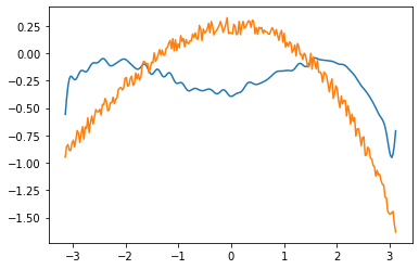
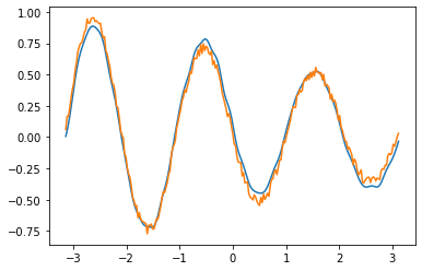
Please note that the arctangent function is applied only in the first and fourth quadrants of the complex plane. There is a clear distinction between periodic and non-periodic approximation. As seen in the examples, dataset 7 exhibits periodicity while dataset 2 does not. Observing the other plots, it becomes evident that the complex approximation is effective only for periodic sound waves.

Data Compression

In certain instances, we encounter an abundance of information when achieving nearly identical results with a reduced dataset is possible. In this context, we apply this concept to our audio signals.

Signal Compression

The function compressSignal is designed to compress an excess of information into the most crucial data. In this function, we specify three variables: \(Y\), \(K\), and \(\phi\). \(Y\) represents a list of data points, \(K\) is the factor by which the data point list is limited, and \(\phi\) (boolean) determines whether we work through phase shifting or using the regular Fourier series. Upon executing this function, we obtain a graph displaying the original data, followed by a graph displaying the compressed data points.

Signal Reconstruction

The function reconstructSignal aims to approximate the original data points from the compressed data points. In this function, we provide four variables: amplitudes, position, quantity_Y, and \(\phi\). amplitudes is the list of \(a_k\) or \(c_k\) values, position is the list of \(b_k\) or phase values, quantity_Y is the number of points to be retrieved, and \(\phi\) represents the phase shift. Upon executing this function, a new list is generated containing the reconstructed amplitudes.

Examples

It is essential to ensure that the written routines cooperate seamlessly. To achieve this, we have opted for a multi-file system. Specifically, we have created two files: TeamG_procedures.py is responsible for the functionality of our program, encompassing all discussed topics along with supplementary components. Additionally, we have created TeamG_examples.py to visualize the described processes. The latter imports the former to utilize its functionality effectively.

Fast Fourier Transform

Fast Fourier Transform

The Fourier transformation is undoubtedly one of the most crucial mathematical concepts in our modern society. We employ such a transformation to create a frequency spectrum from data . These spectra provide us with a wealth of information about an audio signal, enabling complex signal manipulations. A notable example is the removal of noise from audio recordings, achieved by eliminating specific frequencies from the transformation. Furthermore, there exists a method to revert from the transformed function to an audio file. This entire process can be performed using a DFT, which stands for Discrete Fourier Transform. This algorithm takes audio files and performs several mathematical operations to obtain a transformed function.

However, a significant issue arises when running our program. It becomes apparent that it delivers results relatively slowly. This problem becomes especially evident when attempting to analyze longer audio files. This sluggish performance is unacceptable, particularly when dealing with time-sensitive scenarios. The FFT algorithm presents a solution by incorporating various mathematical concepts from linear algebra to expedite the process.

Operation of the FFT

The algorithm operates based on several concepts in linear algebra, aiming to simplify DFT computations. The way DFT operates can be expressed as the following matrix multiplication:

(1) \(\begin{gathered} \begin{Bmatrix} A_{0}\\ A_{1}\\ A_{2}\\ A_{3} \end{Bmatrix} = \begin{Bmatrix} \label{matrix:omega} \omega^{0}&\omega^{0}&\omega^{0}&\omega^{0}\\ \omega^{0}&\omega^{1}&\omega^{2}&\omega^{3}\\ \omega^{0}&\omega^{2}&\omega^{4}&\omega^{6}\\ \omega^{0}&\omega^{3}&\omega^{6}&\omega^{9} \end{Bmatrix} \cdot \begin{Bmatrix} a_{0}\\ a_{1}\\ a_{2}\\ a_{3} \end{Bmatrix} \end{gathered}\)

Here, \(A_{n}\) represents the transformed function value, and \(\omega\) is given by the equation: \(e^{-2\pi i/n}\), where \(n\) is the number of data points, and \(a_{n}\) denotes the data points.

The matrix presented here is small and thus not challenging to compute. However, the situation changes rapidly when we return to reality. Audio files contain a substantial amount of data, resulting in matrices of this kind becoming extremely large. This inevitably leads us to a situation where the time required to calculate this matrix becomes prohibitively long. The FFT offers a solution to this challenge. By applying a set of mathematical principles, we can simplify the problem.

(2) \(\begin{gathered} \label{eq:opsplitsing} \begin{Bmatrix} A_{0}\\ A_{1}\\ A_{2}\\ A_{3} \end{Bmatrix} = \begin{Bmatrix} I_{2} & -D_{2}\\ I_{2} & -D_{2} \end{Bmatrix} \cdot \begin{Bmatrix} F_{2} & 0_{2}\\ 0_{2}& F_{2} \end{Bmatrix} \cdot \begin{Bmatrix} a_{\text{even}}\\ a_{\text{oneven}} \end{Bmatrix} \end{gathered}\)

We observe that the DFT has now been decomposed into several matrices. Among these matrices, we find the identity matrix \(I\) and the zero matrix \(0\). The matrix \(F\) is equivalent to the central matrix mentioned here above (2). Lastly, there is also the matrix \(D\), which is represented as follows:

(3) \(\begin{gathered} \begin{Bmatrix} \omega^{0}&0\\ 0&\omega^{1} \end{Bmatrix} \end{gathered}\)

It is evident that the computations will be significantly faster since numerous terms are eliminated due to the presence of many zeros. Furthermore, the process of decomposition can be repeated. If we start with an \(8\times8\) matrix, we can divide it into a \(4\times4\) matrix, which we can then further decompose following the process described in equation (2).

with \(\begin{gathered} Q_{4} = \begin{Bmatrix} F_{2} & 0_{2}\\ 0_{2}& F_{2} \end{Bmatrix} \end{gathered}\)

Advantages of FFT

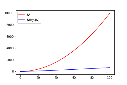
The significant advantage of the FFT is its much faster execution compared to the ordinary DFT. This difference in performance has been quantified by calculating the complexity of the two different algorithms. The complexity of the DFT is \(\mathcal{O}(n^{2})\), which has catastrophic implications for large input lists. Especially when considering that a 5-second audio file already contains 220,000 data points. When comparing this with the complexity of the FFT algorithm , which is \(\mathcal{O}(n\log{}n)\), we observe a significant improvement. The FFT complexity behaves approximately linearly.

Implementation of FFT

As a team, we have also chosen to write a program in Python that demonstrates how the FFT works. The reason for this choice is that the FFT algorithm is so commonly used that a library with FFT functionality exists in a wide range of programming languages. In Python, such an example of a library is called numpy. We use the built-in function, not because it would be too difficult to create one ourselves, but because the intention is to use it. This library is highly optimized to run as efficiently as possible, saving a considerable amount of time for the programmer.

Our program takes an audio file, applies the FFT to it, and then displays the results on a graph. Finally, we take the inverse FFT of our result and export it as a .wav file. We do this to demonstrate that we can seamlessly transition between the data and the transformation. Depending on the purpose of our program, we can make various adjustments to the transformation between these steps. This is also the principle on which technologies like auto-tune operate.

    	# in nemen van bestanden en ze visualiseren
    	path = 'dwarsfluit re.wav'
    	geluidsbestand = innamewav(path)
    	
    	plt.plot(geluidsbestand[0], geluidsbestand[1])
    	plt.title("Origineel geluidsbestand")
    	plt.ylabel("Amplitude")
    	plt.xlabel("Tijd(ms)")
    	plt.show()    
    	
    	
    	# berekenen van de FFT
    	start = time.time()
    	
    	fourier = np.fft.rfft(geluidsbestand[1])
    	
    	stop = time.time()
    	print("het duurde",str(stop - start),"seconden om de fourier transformatie te berekenen.")
    	
    	
    	# Tonen van de FFT
    	plt.plot(abs(fourier))
    	plt.title("Fourier transformatie")
    	plt.xlabel("frequentie")
    	plt.ylabel("amplitude")
    	plt.show()
    	
    	
    	#De omgekeerde fouriertransformatie toepassen
    	
    	omgekeerde = irfft(fourier)
    	
    	plt.plot(omgekeerde)
    	plt.title("Omgekeerde Fourier transformatie")
    	plt.xlabel('datapunten')
    	plt.ylabel("amplitude")
    	plt.show()
    	
    	#Geluidsbestand maken van de inverse FFT
    	write('geluidsbestand.wav', 44000, omgekeerde)
    	print("Het nieuwe geluidsbestand werd opgeslagen!") 	

It is also worth mentioning that our program keeps track of the speed at which the FFT operates. This serves to further emphasize how quickly we can obtain a transformation.

Conclusion

In conclusion, it is evident that implementing a Fourier analysis is not a simple task, as it involves complex mathematical formulas.

Throughout this project, we have learned that the Fourier series is a fundamental part of Fourier analysis and is used to approximate periodic functions as accurately as possible. The Fourier series represents periodic functions as an infinite sum of simpler sinusoidal and cosinusoidal waves. From approximation theory to signal processing, any pattern with a recognizable periodicity can be described using a combination of sinusoidal and cosinusoidal waves. The Fast Fourier Transform (FFT) is a method to improve the efficiency of the Discrete Fourier Transform (DFT). The FFT is capable of achieving results in \(\mathcal{O}(n\log{}n)\) time, thanks to the ability to decompose the DFT into smaller operations, reducing the computational workload.

Authors: Ibrahim El Kaddouri, Mathis Bossuyt, Florijon Sharku, Iben Troch, Emiel Vanspranghels, Robbe Decapmaker, Hendrik Quintelier, Marijn Braem